1.1. Systems of two linear equations and second-order determinants
Consider a system of two linear equations with two unknowns:
Odds  with unknown
  and
and  have two indices: the first indicates the number of the equation, the second - the number of the variable.


Cramer's rule: The solution of the system is found by dividing the auxiliary determinants by the main determinant of the system
 ,
,

Remark 1. The use of Cramer's rule is possible if the determinant of the system  is not equal to zero.
Remark 2. Cramer's formulas can also be generalized to higher order systems.
Example 1 Solve system:  .
.
Solution.
 ;
;
 ;
;
 ;
;

Examination:

Conclusion: The system is correct:  .
.
1.2. Systems of three linear equations and third-order determinants
Consider a system of three linear equations with three unknowns:

The determinant, composed of the coefficients of the unknowns, is called system qualifier or master qualifier:
 .
.
If a  then the system has a unique solution, which is determined by the Cramer formulas:

where are the determinants  are called auxiliary and are obtained from the determinant
  by replacing its first, second, or third column with a column of free system members.
Example 2 Solve the system  .
.
Let's form the main and auxiliary determinants:

It remains to consider the rules for calculating third-order determinants. There are three of them: the column addition rule, the Sarrus rule, and the expansion rule.
a) The rule for adding the first two columns to the main determinant:
![]()
The calculation is carried out as follows: with their sign are the products of the elements of the main diagonal and along the parallels to it, with the opposite sign, they take the products of the elements of the secondary diagonal and along the parallels to it.
b) Sarrus rule:


With their sign, they take the products of the elements of the main diagonal and along the parallels to it, and the missing third element is taken from the opposite corner. With the opposite sign, they take the products of the elements of the secondary diagonal and along the parallels to it, the third element is taken from the opposite corner.
c) The rule of expansion by the elements of a row or column:
If a  , then .
Algebraic addition is a lower order determinant obtained by deleting the corresponding row and column and taking into account the sign  , where
  - line number
  - column number.
For example,
 ,
,
 ,
,
 etc.
etc.
Let us calculate the auxiliary determinants according to this rule  and
and  , expanding them by the elements of the first row.
Having calculated all the determinants, we find the variables according to Cramer's rule:

Examination:

Conclusion: the system is correct: .
Basic properties of determinants
It must be remembered that the determinant is number, found according to some rules. Its calculation can be simplified if we use the basic properties that are valid for determinants of any order.
Property 1. The value of the determinant will not change if all its rows are replaced by corresponding columns and vice versa.

The operation of replacing rows with columns is called transposition. It follows from this property that any statement that is true for the rows of a determinant will also be true for its columns.
Property 2. If two rows (columns) are interchanged in the determinant, then the sign of the determinant will change to the opposite.

Property 3. If all elements of any row of the determinant are equal to 0, then the determinant is equal to 0.
Property 4.
If the elements of the determinant string are multiplied (divided) by some number  , then the value of the determinant will increase (decrease) in
  once.
once.

If the elements of any row have a common factor, then it can be taken out of the determinant sign.

Property 5. If the determinant has two identical or proportional rows, then such a determinant is equal to 0.
Property 6. If the elements of any row of the determinant are the sum of two terms, then the determinant is equal to the sum of the two determinants.

Property 7. The value of the determinant does not change if the elements of a row are added to the elements of another row, multiplied by the same number.
In this determinant, at first the third, multiplied by 2, was added to the second row, then the second was subtracted from the third column, after which the second row was added to the first and third, as a result we got a lot of zeros and simplified the calculation.
Elementary transformations determinant are called its simplifications due to the use of these properties.
Example 1 Compute determinant

Direct counting according to one of the above rules leads to cumbersome calculations. Therefore, it is advisable to use the properties:
a) subtract the second row, multiplied by 2, from the first row;
b) subtract the third row from the second row, multiplied by 3.
As a result, we get:

Let us expand this determinant in terms of the elements of the first column, which contains only one nonzero element.
 .
.
Systems and determinants of higher orders
system  linear equations with
  unknowns can be written as follows:

For this case, it is also possible to compose the main and auxiliary determinants, and determine the unknowns according to Cramer's rule. The problem is that higher order determinants can only be computed by lowering the order and reducing them to third order determinants. This can be done by direct decomposition into row or column elements, as well as by preliminary elementary transformations and further decomposition.
Example 4 Calculate fourth order determinant

Solution find in two ways:
a) by direct expansion over the elements of the first row:

b) by preliminary transformations and further decomposition
|
|
a) subtract line 3 from line 1 |
|
|
b) add line II to line IV |


Example 5 Calculate fifth order determinant, getting zeros in third row using fourth column
|
|
subtract the second from the first row, subtract the second from the third, and subtract the second multiplied by 2 from the fourth. |


subtract the third from the second column: 
subtract the third from the second row: 
Example 6 Solve system:

Solution. Let us compose the determinant of the system and, applying the properties of the determinants, calculate it:

(from the first row we subtract the third, and then in the resulting third-order determinant from the third column we subtract the first, multiplied by 2). Determinant  , therefore, Cramer's formulas are applicable.
Let's calculate the rest of the determinants:


The fourth column is multiplied by 2 and subtracted from the rest


The fourth column was subtracted from the first, and then, multiplied by 2, subtracted from the second and third columns.


 .
.
Here, the same transformations were performed as for  .
.

 .
.
When found  the first column was multiplied by 2 and subtracted from the rest.
According to Cramer's rule, we have:
After substituting the found values into the equations, we make sure that the solution of the system is correct.
2. MATRIXES AND THEIR USE
IN SOLVING SYSTEMS OF LINEAR EQUATIONS
Lecture 1.1.Numerical matrices and operations on them.
Summary:The place of linear algebra and analytic geometry in natural science. The role of domestic scientists in the development of these sciences. The concept of a matrix. Operations on matrices and their properties.
A table of numbers of the form is called a rectangular matrix dimensions . Matrices are denoted by capital Latin letters A, B, C ... The numbers that make up the table are called elements matrices. Each element has two indexes and denoting, respectively, the number of the row () and the number of the column () in which the given element is located. The following matrix notation is used.
The two matrices are called equal , if they have the same dimension (i.e., the same number of rows and columns) and if the numbers in the corresponding places of these matrices are equal.
If the number of rows of a matrix is equal to the number of columns, then the matrix is called square
. In a square matrix, the number of rows (or columns) is called the order of the matrix. In particular, a first-order square matrix is just a real number. Accordingly, they say that vector string
![]() is a matrix of dimension , and column vector
has dimension .
is a matrix of dimension , and column vector
has dimension .
The elements on the main diagonal of a square matrix (going from the upper left to the lower right corner) are called diagonal .
A square matrix with all elements not on the main diagonal equal to 0 is called diagonal .
A diagonal matrix in which all diagonal entries are 1 and all off-diagonal entries are 0 is called single and is denoted by or , where n is its order.
The main operations on matrices are matrix addition and matrix multiplication by a number.
work matrices BUT a number is called a matrix of the same dimension as the matrix BUT, each element of which is multiplied by this number.

For example: ![]() ;
; ![]() .
.
Properties of the operation of multiplying a matrix by a number:
1.l(m BUT )=(lm) BUT (associativity)
2.l( BUT +AT )=l BUT +l AT (distributivity with respect to matrix addition)
3. (l+m) BUT =)=l BUT +m BUT (distributivity with respect to addition of numbers)
Linear combination of matrices BUT and AT of the same size is called an expression of the form: a BUT +b AT , where a,b are arbitrary numbers
sum matrix and AT (this action is applicable only to matrices of the same dimension) is called a matrix FROM of the same dimension, the elements of which are equal to the sums of the corresponding elements of the matrices BUT and AT .


Matrix addition properties:
1)BUT +AT =AT +BUT (commutativity)
2)(BUT +AT )+FROM =BUT +(AT +FROM )=BUT +AT +FROM (associativity)
Difference matrix and AT (this action is applicable only to matrices of the same dimension) is called a matrix C of the same dimension, the elements of which are equal to the difference of the corresponding elements of the matrices BUT and AT .


Transposition. If the elements of each row of the dimension matrix are written in the same order in the columns of the new matrix, and the column number is equal to the row number, then the new matrix is called transposed with respect to and denoted by . The dimension is equal. The transition from to is called transposition. It is also clear that .  ,
, 
Matrix multiplication. The operation of matrix multiplication is possible only if the number of columns of the first factor is equal to the number of rows of the second. As a result of multiplication, we get a matrix, the number of rows of which coincides with the number of rows of the first multiplier, and the number of columns with the number of columns of the second: ![]()
Matrix multiplication rule: to get the element in the -th row and -th column of the product of two matrices, you need to multiply the elements of the -th row of the first matrix by the elements of the -th column of the second matrix and add the resulting products. In mathematical jargon, they sometimes say: you need to multiply the -th row of the matrix by the -th column of the matrix. It is clear that the row of the first and the column of the second matrix must contain the same number of elements.
In contrast to these operations, the operation of multiplying a matrix by a matrix is more difficult to define. Let two matrices be given BUT and AT , and the number of columns of the first of them is equal to the number of rows of the second: for example, the matrix BUT has dimension , and the matrix AT - dimension . If a
 ,
,  , then the matrix of dimension
 , where (i=1,…,m;j=1,…,k)
is called the matrix product BUT to matrix AT and denoted AB .
Properties of the operation of matrix multiplication:
1. (AB)C=A(BC)=ABC (associativity)
2. (A+B)C=AC+BC (distributivity)
3. A(B+C)=AB+A (distributivity)
4. Matrix multiplication is noncommutative: AB not equal VA ., if equal, then these matrices are called commutative.
Elementary transformations over matrices:
1. Swap two rows (columns)
2. Multiplying a row (column) by a non-zero number
3. Adding to the elements of one row (column) the elements of another row (column), multiplied by any number
Lecture 1.2.Determinants with real coefficients. Finding the inverse matrix.
Summary:Determinants and their properties. Methods for calculating determinants with real coefficients. Finding the inverse matrix for third-order matrices.
The concept of a determinant is introduced only for a square matrix. Determinant - this is number, which is found according to well-defined rules and is denoted or det A .
Determinant matrices second order located like this: or
Third order determinant number is called:
 .
.
To remember this cumbersome formula, there is a "rule of triangles":
You can also calculate by another method - the method of expansion by row or by column. Let us introduce some definitions:
Minor square matrix BUT
is called the matrix determinant BUT
, which is obtained by deleting the -th row and -th column: for example, for a minor - ![]() .
.
Algebraic addition element of the determinant is called its minor, taken with its sign if the sum of the numbers of the row and column in which the element is located is even, and with the opposite sign if the sum of the numbers is odd: .
Then: Third order determinant is equal to the sum of the products of the elements of some column (row) and their algebraic complements.
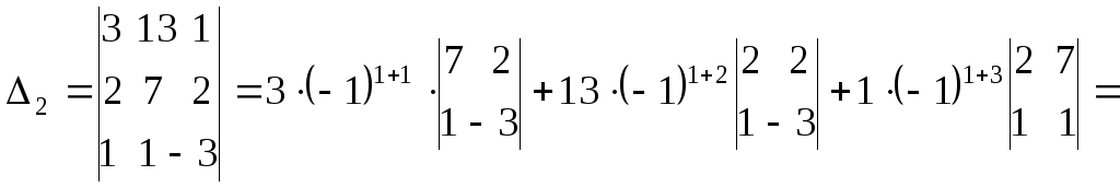
PR: Calculate the determinant: by expanding it over the elements of the first row.
![]()
Properties of determinants:
1. The determinant is 0 if it contains two identical rows (columns) or a zero row (column).
2. The determinant changes its sign when two rows (columns) are interchanged.
3. The common factor in a row (in a column) can be taken out of the sign of the determinant.
4. The determinant does not change if any other row (another column) multiplied by an arbitrary number is added to a row (column).
5. The determinant does not change when the matrix is transposed.
6. The identity matrix determinant is 1:
7. The determinant of the product of matrices is equal to the product of the determinants
inverse matrix.
The square matrix is called non-degenerate if its determinant is non-zero.
If when multiplying square matrices BUT and AT in any order, the identity matrix is obtained ( AB=BA=E ), then the matrix AT is called the inverse matrix for the matrix BUT and is denoted by , i.e. .
Theorem.Every non-singular matrix has an inverse.
Algorithm for finding the inverse matrix:
Inverse matrix. A square matrix is called nondegenerate if its determinant is nonzero. Otherwise, it is called degenerate. .
The matrix inverse to a matrix is denoted by . If an inverse matrix exists, then it is unique and ![]()
Where is the adjoint (union), composed of algebraic complements j: 
Then the determinant of the inverse matrix is related to the determinant of this matrix by the following relationship: . Indeed, ![]() , whence this equality follows.
, whence this equality follows.
Inverse Matrix Properties:
1. ![]() , where are nonsingular square matrices of the same order.
, where are nonsingular square matrices of the same order.
3. ![]() .
.
4. ![]()
Lecture 1.3.Solving systems of linear equations by the Cramer method. Gauss methods and matrix calculus.
Summary:Cramer's method and Gauss's method for solving systems of linear algebraic equations. Matrix method for solving systems of equations. Matrix rank. The Kronecker-Capelli theorem. Fundamental decision system. Homogeneous and inhomogeneous systems.
The system of equations of the following form:
 (*) , where , are coefficients, are variables, is called system of linear equations. To solve a system of linear equations means to indicate all solutions of the system, i.e. such sets of variable values that turn the equations of the system into identities. The system of linear equations is called.
KOSTROMA BRANCH OF THE MILITARY UNIVERSITY OF RCHB PROTECTION
Department of "Automation of command and control"
Only for teachers
"I approve"
Head of Department No. 9
Colonel YAKOVLEV A.B.
"____" ______________ 2004
Associate Professor A.I. Smirnova
"DETERMINERS.
SOLUTION OF SYSTEMS OF LINEAR EQUATIONS"
LECTURE № 2 / 1
Discussed at the meeting of the department No. 9
"____" ___________ 2004
Protocol No. ___________
Kostroma, 2004.
Introduction
1. Determinants of the second and third order.
2. Properties of determinants. Decomposition theorem.
3. Cramer's theorem.
Conclusion
Literature
1. V.E. Schneider et al., A Short Course in Higher Mathematics, Volume I, Ch. 2, item 1.
2. V.S. Shchipachev, Higher Mathematics, ch.10, p.2.
INTRODUCTION
The lecture deals with determinants of the second and third orders, their properties. As well as Cramer's theorem, which allows solving systems of linear equations using determinants. Determinants are also used later in the topic "Vector Algebra" when calculating the cross product of vectors.
1st study question QUALIFIERS OF THE SECOND AND THIRD
ORDER
Consider a table of four numbers of the form
The numbers in the table are denoted by a letter with two indices. The first index indicates the row number, the second index indicates the column number.
DEFINITION 1. Second order determinant called expression kind :
 (1)
(1)
Numbers a 11, …, a 22 are called the elements of the determinant.
Diagonal formed by elements a 11 ; a 22 is called the main, and the diagonal formed by the elements a 12 ; a 21 - on the side.
Thus, the second-order determinant is equal to the difference between the products of the elements of the main and secondary diagonals.
Note that the answer is a number.
EXAMPLES. Calculate:

Consider now a table of nine numbers written in three rows and three columns:

DEFINITION 2. Third order determinant is called an expression of the form :
Elements a 11; a 22 ; a 33 - form the main diagonal.
Numbers a 13; a 22 ; a 31 - form a side diagonal.
Let us depict, schematically, how the terms with plus and minus are formed:
 " + " " – "
Plus includes: the product of the elements on the main diagonal, the other two terms are the product of the elements located at the vertices of triangles with bases parallel to the main diagonal.
Terms with a minus are formed in the same way with respect to the secondary diagonal.
This rule for calculating the third order determinant is called
right
EXAMPLES. Calculate by the rule of triangles:

COMMENT. Determinants are also called determinants.
2nd study question PROPERTIES OF DETERMINERS.
EXPANSION THEOREM
Property 1. The value of the determinant will not change if its rows are interchanged with the corresponding columns.
 .
.
Expanding both determinants, we are convinced of the validity of equality.
Property 1 sets the equality of rows and columns of the determinant. Therefore, all further properties of the determinant will be formulated for both rows and columns.
Property 2. When two rows (or columns) are interchanged, the determinant changes sign to the opposite, preserving the absolute value .
 .
.
Property 3. Common multiplier of row elements (or column)can be taken out of the sign of the determinant.
 .
.
Property 4. If the determinant has two identical rows (or columns), then it is equal to zero.

This property can be proved by direct verification, or property 2 can be used.
Denote the determinant by D. When two identical first and second rows are interchanged, it will not change, and by the second property it must change sign, i.e.
D = - DÞ 2 D = 0 ÞD = 0.
Property 5. If all elements of some string (or column)are zero, then the determinant is zero.
This property can be considered as a special case of property 3 with
Property 6. If the elements of two rows (or columns)determinant are proportional, then the determinant is zero.
 .
.
It can be proved by direct verification or by using properties 3 and 4.
Property 7. The value of the determinant does not change if the elements of any row (or column) are added to the corresponding elements of another row (or column), multiplied by the same number.
 .
.
It is proved by direct verification.
The use of these properties can in some cases facilitate the process of calculating determinants, especially of the third order.
For what follows, we need the concepts of minor and algebraic complement. Consider these concepts to define the third order.
DEFINITION 3. Minor of a given element of a third-order determinant is called a second-order determinant obtained from a given one by deleting the row and column at the intersection of which the given element stands.
Element minor a i j denoted M i j. So for element a 11 minor

It is obtained by deleting the first row and the first column in the third-order determinant.
DEFINITION 4. Algebraic complement of the determinant element call it a minor multiplied by (-1)k , where k - the sum of the row and column numbers at the intersection of which the given element is located.
Algebraic element addition a i j denoted BUT i j .
In this way, BUT i j =
.Let us write out the algebraic complements for the elements a 11 and a 12.
 .
.
.
.
It is useful to remember the rule: the algebraic complement of an element of a determinant is equal to its signed minor a plus, if the sum of the row and column numbers in which the element is located, even, and with sign minus if this amount odd .
In the course of solving problems in higher mathematics, it is very often necessary to calculate matrix determinant. The matrix determinant appears in linear algebra, analytic geometry, mathematical analysis and other branches of higher mathematics. Thus, one simply cannot do without the skill of solving determinants. Also, for self-testing, you can download the determinant calculator for free, it will not teach you how to solve determinants by itself, but it is very convenient, because it is always beneficial to know the correct answer in advance!
I will not give a strict mathematical definition of the determinant, and, in general, I will try to minimize mathematical terminology, this will not make it easier for most readers. The purpose of this article is to teach you how to solve second, third and fourth order determinants. All the material is presented in a simple and accessible form, and even a full (empty) kettle in higher mathematics, after careful study of the material, will be able to correctly solve the determinants.
In practice, most often you can find a second-order determinant, for example: , and a third-order determinant, for example:  .
.
Fourth order determinant  is also not an antique, and we will come to it at the end of the lesson.
I hope everyone understands the following: The numbers inside the determinant live on their own, and there is no question of any subtraction! You can't swap numbers!
(In particular, it is possible to perform pairwise permutations of the rows or columns of the determinant with a change in its sign, but often this is not necessary - see the next lesson Properties of the determinant and lowering its order)
Thus, if any determinant is given, then do not touch anything inside it!
Notation: If given a matrix ![]() , then its determinant is denoted by . Also, very often the determinant is denoted by a Latin letter or Greek.
, then its determinant is denoted by . Also, very often the determinant is denoted by a Latin letter or Greek.
1)What does it mean to solve (find, reveal) a determinant? To calculate the determinant is to FIND THE NUMBER. The question marks in the above examples are completely ordinary numbers.
2) Now it remains to figure out HOW to find this number? To do this, you need to apply certain rules, formulas and algorithms, which will be discussed now.
Let's start with the determinant "two" to "two":
![]()
THIS SHOULD BE REMEMBERED, at least for the time of studying higher mathematics at the university.
Let's look at an example right away:
Ready. Most importantly, DO NOT CONFUSE THE SIGNS.
Three-by-three matrix determinant can be opened in 8 ways, 2 of them are simple and 6 are normal.
Let's start with two simple ways
Similar to the “two by two” determinant, the “three by three” determinant can be expanded using the formula:


The formula is long and it is easy to make a mistake due to inattention. How to avoid embarrassing mistakes? For this, a second method for calculating the determinant was invented, which actually coincides with the first. It is called the Sarrus method or the "parallel strips" method.
The bottom line is that the first and second columns are attributed to the right of the determinant and the lines are carefully drawn with a pencil:

Factors located on the "red" diagonals are included in the formula with a "plus" sign.
Factors located on the "blue" diagonals are included in the formula with a minus sign:
Example:


Compare the two solutions. It is easy to see that this is the SAME, just in the second case the factors of the formula are slightly rearranged, and, most importantly, the probability of making a mistake is much less.
Now consider the six normal ways to calculate the determinant
Why normal? Because in the vast majority of cases, determinants need to be opened in this way.
As you can see, the three-by-three determinant has three columns and three rows.
You can solve the determinant by expanding it on any row or on any column.
Thus, it turns out 6 ways, while in all cases using of the same type algorithm.
The matrix determinant is equal to the sum of the products of the row (column) elements and the corresponding algebraic additions. Scary? Everything is much simpler, we will use an unscientific, but understandable approach, accessible even to a person who is far from mathematics.
In the following example, we will expand the determinant on the first line.
To do this, we need a matrix of signs: . It is easy to see that the signs are staggered.
Attention! The matrix of signs is my own invention. This concept is not scientific, it does not need to be used in the final design of assignments, it only helps you understand the algorithm for calculating the determinant.
I'll give the complete solution first. Again, we take our experimental determinant and perform calculations:

And the main question: HOW to get this from the “three by three” determinant: ![]() ?
?
So, the “three by three” determinant comes down to solving three small determinants, or as they are also called, MINORS. I recommend remembering the term, especially since it is memorable: minor - small.
As soon as the method of expansion of the determinant is chosen on the first line, obviously everything revolves around it:
Elements are usually viewed from left to right (or top to bottom if a column would be selected)
Let's go, first we deal with the first element of the string, that is, with the unit:
1) We write out the corresponding sign from the matrix of signs: 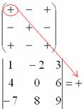
2) Then we write the element itself: 
3) MENTALLY cross out the row and column in which the first element is: 
The remaining four numbers form the determinant "two by two", which is called MINOR given element (unit).
We pass to the second element of the line.
4) We write out the corresponding sign from the matrix of signs:

5) Then we write the second element: 
6) MENTALLY cross out the row and column containing the second element: 
Well, the third element of the first line. No originality
7) We write out the corresponding sign from the matrix of signs: 
8) Write down the third element: 
9) MENTALLY cross out the row and column in which the third element is: 
The remaining four numbers are written in a small determinant.
The rest of the steps are not difficult, since we already know how to count the “two by two” determinants. DO NOT CONFUSE THE SIGNS!
Similarly, the determinant can be expanded over any row or over any column. Naturally, in all six cases the answer is the same.
The determinant "four by four" can be calculated using the same algorithm.
In this case, the matrix of signs will increase:

In the following example, I expanded the determinant on the fourth column:

And how it happened, try to figure it out on your own. More information will come later. If anyone wants to solve the determinant to the end, the correct answer is: 18. For training, it is better to open the determinant in some other column or other line.
To practice, to reveal, to make calculations is very good and useful. But how much time will you spend on a big determinant? Isn't there a faster and more reliable way? I suggest that you familiarize yourself with effective methods for calculating determinants in the second lesson - Determinant properties. Reducing the order of the determinant.
BE CAREFUL!


