- Systems m linear equations With n unknown.
Solving a system of linear equations- this is such a set of numbers ( x 1 , x 2 , …, x n), when substituted into each of the equations of the system, the correct equality is obtained.
Where a ij , i = 1, …, m; j = 1, …, n— system coefficients;
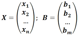
b i , i = 1, …, m- free members;
x j , j = 1, …, n- unknown.
The above system can be written in matrix form: A X = B,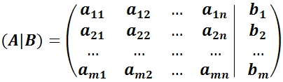
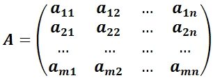
Where ( A|B) is the main matrix of the system;
A— extended system matrix;
X— column of unknowns;
B— column of free members.
If matrix B is not a null matrix ∅, then this system linear equations is called inhomogeneous.
If matrix B= ∅, then this system of linear equations is called homogeneous. A homogeneous system always has a zero (trivial) solution: x 1 = x 2 = …, x n = 0.
Joint system of linear equations is a system of linear equations that has a solution.
Inconsistent system of linear equations is an unsolvable system of linear equations.
A certain system of linear equations is a system of linear equations that has a unique solution.
Indefinite system of linear equations is a system of linear equations with an infinite number of solutions. - Systems of n linear equations with n unknowns
If the number of unknowns is equal to the number of equations, then the matrix is square. The determinant of a matrix is called the main determinant of a system of linear equations and is denoted by the symbol Δ.
Cramer method for solving systems n linear equations with n unknown.
Cramer's rule.
If the main determinant of a system of linear equations is not equal to zero, then the system is consistent and defined, and the only solution is calculated using the Cramer formulas:
where Δ i are determinants obtained from the main determinant of the system Δ by replacing i th column to the column of free members. . - Systems of m linear equations with n unknowns
Kronecker–Capelli theorem.
In order for a given system of linear equations to be consistent, it is necessary and sufficient that the rank of the system matrix be equal to the rank of the extended matrix of the system, rang(Α) = rang(Α|B).
If rang(Α) ≠ rang(Α|B), then the system obviously has no solutions.
If rang(Α) = rang(Α|B), then two cases are possible:
1) rank(Α) = n(number of unknowns) - the solution is unique and can be obtained using Cramer’s formulas;
2) rank(Α)< n - there are infinitely many solutions. - Gauss method for solving systems of linear equations
Let's create an extended matrix ( A|B) of a given system from the coefficients of the unknowns and the right-hand sides.
The Gaussian method or the method of eliminating unknowns consists of reducing the extended matrix ( A|B) using elementary transformations over its rows to a diagonal form (to the upper triangular form). Returning to the system of equations, all unknowns are determined.
TO elementary transformations above the lines are the following:
1) swap two lines;
2) multiplying a string by a number other than 0;
3) adding another string to a string, multiplied by an arbitrary number;
4) throwing out a zero line.
An extended matrix reduced to diagonal form corresponds to a linear system equivalent to the given one, the solution of which does not cause difficulties. . - System of homogeneous linear equations.
A homogeneous system has the form:
corresponds to it matrix equation A X = 0.
1) A homogeneous system is always consistent, since r(A) = r(A|B), there is always a zero solution (0, 0, …, 0).
2) In order for a homogeneous system to have a non-zero solution, it is necessary and sufficient that r = r(A)< n , which is equivalent to Δ = 0.
3) If r< n , then obviously Δ = 0, then free unknowns arise c 1 , c 2 , …, c n-r, the system has non-trivial solutions, and there are infinitely many of them.
4) General solution X at r< n can be written in matrix form as follows:
X = c 1 X 1 + c 2 X 2 + … + c n-r X n-r,
where are the solutions X 1, X 2, …, X n-r form a fundamental system of solutions.
5) The fundamental system of solutions can be obtained from general solution homogeneous system: ,
,
if we sequentially set the parameter values equal to (1, 0, …, 0), (0, 1, …, 0), …, (0, 0, …, 1).
Expansion of the general solution in terms of the fundamental system of solutions is a record of a general solution in the form of a linear combination of solutions belonging to the fundamental system.
Theorem. In order for a system of linear homogeneous equations to have a non-zero solution, it is necessary and sufficient that Δ ≠ 0.
So, if the determinant Δ ≠ 0, then the system has a unique solution.
If Δ ≠ 0, then the system of linear homogeneous equations has an infinite number of solutions.
Theorem. In order for a homogeneous system to have a nonzero solution, it is necessary and sufficient that r(A)< n .
Proof:
1) r there can't be more n(the rank of the matrix does not exceed the number of columns or rows);
2) r< n , because If r = n, then the main determinant of the system Δ ≠ 0, and, according to Cramer’s formulas, there is a unique trivial solution x 1 = x 2 = … = x n = 0, which contradicts the condition. Means, r(A)< n .
Consequence. In order for a homogeneous system n linear equations with n unknowns had a non-zero solution, it is necessary and sufficient that Δ = 0.
Answer: Cramer's method is based on the use of determinants in solving systems of linear equations. This significantly speeds up the solution process.
Definition. A determinant made up of coefficients for unknowns is called a determinant of the system and is denoted (delta).
Determinants
are obtained by replacing the coefficients of the corresponding unknowns with free terms:
 ;
;
 .
.
Cramer formulas for finding unknowns:
![]() .
.
Finding the values of and is possible only if
This conclusion follows from the following theorem.
Cramer's theorem. If the determinant of the system is nonzero, then the system of linear equations has one unique solution, and the unknown is equal to the ratio of the determinants. The denominator contains the determinant of the system, and the numerator contains the determinant obtained from the determinant of the system by replacing the coefficients of this unknown with free terms. This theorem holds for a system of linear equations of any order.
Example 1. Solve a system of linear equations:
According to Cramer's theorem we have:


So, the solution to system (2):
9.operations on sets. Vien diagrams.
Euler-Venn diagrams are geometric representations of sets. The construction of the diagram consists of drawing a large rectangle representing the universal set U, and inside it - circles (or some other closed figures) representing the sets. The figures should intersect in the most general case required in the task and must be labeled accordingly. Points lying inside different areas of the diagram can be considered as elements of the corresponding sets. With the diagram constructed, you can shade certain areas to indicate newly formed sets.
Set operations are considered to obtain new sets from existing ones.
Definition. The union of sets A and B is a set consisting of all those elements that belong to at least one of the sets A, B (Fig. 1):
Definition. The intersection of sets A and B is a set consisting of all those and only those elements that belong simultaneously to both set A and set B (Fig. 2):
Definition. The difference between sets A and B is the set of all those and only those elements of A that are not contained in B (Fig. 3):
 Definition. The symmetric difference of sets A and B is the set of elements of these sets that belong either only to set A or only to set B (Fig. 4):
11. mapping (function), domain of definition, images of sets during mapping, set of values of a function and its graph.
Answer: A mapping from a set E to a set F, or a function defined on E with values in F, is a rule or law f, which assigns each element a certain element.
An element is called an independent element, or an argument of a function f, an element is called a value of a function f, or an image; in this case, the element is called the preimage of the element.
A mapping (function) is usually denoted by the letter f or the symbol, indicating that f maps the set E to F. The notation is also used, indicating that an element x corresponds to an element f(x). Sometimes it is convenient to define a function through an equality that contains a correspondence law. For example, one can say that "the function f is defined by the equality ". If “y” is the general name of the elements of the set F, i.e. F = (y), then the mapping is written in the form of equality y = f(x) and we say that this mapping is specified explicitly.
2. Image and inverse image of a set under a given mapping
Let a mapping and a set be given.
The set of elements from F, each of which is the image of at least one element from D under the mapping f, is called the image of the set D and is denoted by f(D).
Obviously, .
Let now the set be given.
The set of elements such that , is called the inverse image of the set Y under the mapping f and is denoted by f -1 (Y).
If, then. If for each the set f -1 (y) consists of at most one element , then f is called a one-to-one mapping from E to F. However, it is possible to define a one-to-one mapping f of the set E onto F.
The display is called:
Injective (or injection, or one-to-one mapping of the set E into F) if , or if the equation f(x) = y has at most one solution;
Surjective (or surjection, or mapping of a set E onto F) if f(E) = F and if the equation f(x) = y has at least one solution;
Bijective (or bijection, or one-to-one mapping of a set E onto F) if it is injective and surjective, or if the equation f(x) = y has one and only one solution.
3. Superposition of mappings. Inverse, parametric and implicit mappings
1) Let and . Since , the mapping g assigns a specific element to each element.
Thus, each element is assigned by means of a rule
This defines a new mapping (or new feature), which we call a composition of mappings, or a superposition of mappings, or a complex mapping.
2) Let be a bijective mapping and F = (y). Due to the bijectivity of f, each corresponds to a unit image x, which we denote by f -1 (y), and such that f(x) = y. Thus, a mapping is defined, which is called the inverse of the mapping f, or the inverse function of the function f.
Obviously, the mapping f is the inverse of the mapping f -1 . Therefore, the mappings f and f -1 are called mutually inverse. The relations are valid for them
and at least one of these mappings, for example, is bijective. Then there is an inverse mapping, which means .
A mapping defined in this way is said to be defined parametrically using mappings; and the variable from is called a parameter.
4) Let a mapping be defined on a set, where the set contains the zero element. Let us assume that there are sets such that for each fixed equation has a unique solution. Then on the set E it is possible to define a mapping that assigns to each one the value that, for a given x, is a solution to the equation.
Regarding the so defined mapping
it is said to be given implicitly by the equation .
5) A mapping is called a continuation of the mapping , and g is a restriction of the mapping f if and .
The restriction of a mapping to a set is sometimes denoted by the symbol .
6) A display graph is a set
It's clear that .
12. monotonic functions. Inverse function, existence theorem. Functions y=arcsinx y=arcos x x properties and graphs.
Answer: A monotonic function is a function whose increment does not change sign, that is, it is either always non-negative or always non-positive. If, in addition, the increment is not zero, then the function is called strictly monotonic.
Let there be a function f(x) defined on the interval
then they say that on the segment
Note the difference between this definition and the definition of whether a segment is full
Usually, when talking about the inverse function, they replace x with y and y with x(x "y) and write y=f (-1) (x). It is obvious that the original function f(x) and the inverse function f (-1) (x) satisfy the relation
f (-1) (f(x))=f(f (-1) (x))=x.
The graphs of the original and inverse functions are obtained from each other by mirror image relative to the bisector of the first quadrant.
Theorem. Let the function f(x) be defined, continuous and strictly monotonically increasing (decreasing) on the interval. Then the inverse function f (-1) (x) is defined on the segment, which is also continuous and strictly monotonically increases (decreases).
Proof.
Let us prove the theorem for the case when f(x) strictly monotonically increases.
1. Existence of an inverse function.
Since, by the conditions of the theorem, f(x) is continuous, then, according to the previous theorem, the segment is filled entirely. It means that.
Let us prove that x is unique. Indeed, if we take x’>x, then f(x’)>f(x)=y and therefore f(x’)>y. If we take x'' 2. Monotonicity of the inverse function. Let's make the usual replacement x «y and write y= f (-1) (x). This means that x=f(y). Let x 1 >x 2 . Then: y 1 = f (-1) (x 1); x 1 =f(y 1) y 2 = f (-1) (x 2); x 2 =f(y 2) What is the relationship between y 1 and y 2? Let's check the possible options. a) y 1 b) y 1 =y 2? But then f(y 1)=f(y 2) and x 1 =x 2, and we had x 1 >x 2. c) The only option left is y 1 >y 2, i.e. But then f (-1) (x 1)>f (-1) (x 2), and this means that f (-1) (...) strictly monotonically increases. 3. Continuity of the inverse function. Because the values of the inverse function fill the entire segment, then by the previous theorem f (-1) (...) is continuous.< <="" a="" style="color: rgb(255, 68, 0);"> <="" a="" style="color: rgb(0, 0, 0); font-family: Arial; font-size: 11px; font-style: normal; font-variant: normal; font-weight: normal; letter-spacing: normal; line-height: normal; orphans: auto; text-align: start; text-indent: 0px; text-transform: none; white-space: normal; widows: auto; word-spacing: 0px; -webkit-text-stroke-width: 0px; background-color: rgb(0, 171, 160);">
<="" a="" style="color: rgb(255, 68, 0); font-family: Arial; font-size: 11px; font-style: normal; font-variant: normal; font-weight: normal; letter-spacing: normal; line-height: normal; orphans: auto; text-align: start; text-indent: 0px; text-transform: none; white-space: normal; widows: auto; word-spacing: 0px; -webkit-text-stroke-width: 0px; background-color: rgb(0, 171, 160);"> 13.composition of functions. Elementary functions. Functions y=arctg x, y = arcctg x, their properties and graphs. Answer: In mathematics, the composition of functions (superposition of functions) is the application of one function to the result of another. The composition of functions G and F is usually denoted G∘F, which denotes the application of a function G to the result of a function F. Let F:X→Y and G:F(X)⊂Y→Z be two functions. Then their composition is the function G∘F:X→Z, defined by the equality: (G∘F)(x)=G(F(x)),x∈X. Elementary functions are functions that can be obtained using a finite number of arithmetic operations and compositions from the following basic elementary functions: Each elementary function can be specified by a formula, that is, a set of a finite number of symbols corresponding to the operations used. All elementary functions are continuous in their domain of definition. Sometimes the basic elementary functions also include hyperbolic and inverse hyperbolic functions, although they can be expressed through the basic elementary functions listed above. <="" a="" style="color: rgb(255, 68, 0); font-family: Arial; font-size: 11px; font-style: normal; font-variant: normal; font-weight: normal; letter-spacing: normal; line-height: normal; orphans: auto; text-align: start; text-indent: 0px; text-transform: none; white-space: normal; widows: auto; word-spacing: 0px; -webkit-text-stroke-width: 0px; background-color: rgb(0, 171, 160);"> Second order determinant
and is calculated according to the rule Numbers The concept of a third-order determinant is introduced similarly. Third order determinant
is the number that is represented by the symbol and is calculated according to the rule Diagonal formed by elements To remember which products on the right side of equality (1) are taken with the sign “ You can introduce the concept of a determinant of the 4th, 5th, etc. orders. Minor
Algebraic complement
Properties of determinants. The value of the determinant will not change if its rows and columns are swapped. The operation in question is called transposition. Property 1 establishes equality of rows and columns of the determinant. Task 1. Calculate determinants: Task 2. Calculate the determinants by decomposing them into the elements of the first column: 1)
Task 3. Find 1)
I) System of two linear inhomogeneous equations with two unknowns Let's denote a) If the determinant of the system b) If the determinant of the system 1)
2) if at least one of the determinants II) System of two linear homogeneous equations with three variables The linear equation is called homogeneous
, if the free term of this equation is equal to zero. and if b) If the condition III) A system of three linear inhomogeneous equations with three unknowns: Let's compose and calculate the main determinant and if b) If 1)
2) at least one of the determinants IV) A system of three linear homogeneous equations with three unknowns: This system is always consistent because it has a zero solution. a) If the determinant of the system b) If Task 4. Solve system of equations Solution. Let's calculate the determinant of the system Because Task 5. Solve system of equations Solution. Let us calculate the determinant of the system: Consequently, a system of homogeneous equations has infinitely many non-zero solutions. We solve the system of the first two equations (the third equation is their consequence): Let's move the variable From here, using formulas (1) we obtain Problems to solve independently Task 6. Solve using determinants of the system of equations: 1)
2)
3)
4) 5)
6)
7)
8)
9)
10)
11)
12)
A matrix is a rectangular table made up of numbers. Let a square matrix of order 2 be given: The determinant (or determinant) of order 2 corresponding to a given matrix is the number A 3rd order determinant (or determinant) corresponding to a matrix is a number Example 1: Find determinants of matrices and System of linear algebraic equations Let a system of 3 linear equations with 3 unknowns be given System (1) can be written in matrix-vector form where A is the coefficient matrix B - extended matrix X is the required component vector; Let a system of linear equations with two unknowns be given: Let's consider solving systems of linear equations with two and three unknowns using Cramer's formulas. Theorem 1. If the main determinant of the system is different from zero, then the system has a solution, and a unique one. The solution of the system is determined by the formulas: where x1, x2 are the roots of the system of equations, The main determinant of the system, x1, x2 are auxiliary determinants. Auxiliary qualifiers: Solving systems of linear equations with three unknowns using Cramer's method. Let a system of linear equations with three unknowns be given: Theorem 2. If the main determinant of the system is different from zero, then the system has a solution, and a unique one. The solution of the system is determined by the formulas: where x1, x2, x3 are the roots of the system of equations, The main determinant of the system, x1, x2, x3 are auxiliary determinants. The main determinant of the system is determined by: Auxiliary qualifiers: 1. Determinants of the second and third orders and their properties 1.1. The concept of a matrix and a second-order determinant
A rectangular table of numbers containing an arbitrary number m rows and an arbitrary number of columns is called a matrix. To indicate matrices use either double vertical bars or round ones brackets. For example: 28 20 18 28 20 18 If the number of rows of a matrix coincides with the number of its columns, then the matrix called square. The numbers that make up the matrix call it elements. Consider a square matrix consisting of four elements: The second-order determinant corresponding to matrix (3.1), is a number equal to - and denoted by the symbol So, by definition The elements that make up the matrix of a given determinant are usually are called elements of this determinant. The following statement is true: in order for the determinant second order was equal to zero, it is necessary and sufficient that the elements of its rows (or, correspondingly, its columns) were proportional. To prove this statement, it is enough to note that each from the proportions / = / and / = / is equivalent to the equality = , and the last equality in force (3.2) is equivalent to the vanishing of the determinant. 1.2. System of two linear equations in two unknowns
Let us show how second-order determinants are used for research and finding solutions to a system of two linear equations with two unknowns (coefficients and free terms are considered in this case given). Recall that a pair of numbers is called a solution to system (3.3), if substitution of these numbers in place and into the given system turns both equation (3.3) into identities. Multiplying the first equation of system (3.3) by -, and the second by - and then adding up the resulting equalities, we get Similarly, by multiplying equations (3.3) by - and accordingly Let us introduce the following notation: = , = , = . (3.6) Using these notations and the expression for the determinant of the second order of magnitude, equations (3.4) and (3.5) can be rewritten as: Determinant composed of coefficients for unknowns system (3.3) is usually called determinant of this system. notice, that determinants and are obtained from the determinant of the system by replacing its first or second column, respectively, by free terms. Two cases may arise: 1) the determinant of the system is different from zero; 2) this determinant is equal to zero. Let us first consider case 0. From equations (3.7) we immediately obtain formulas for unknowns, called Cramer formulas: The resulting Cramer formulas (3.8) give a solution to system (3.7) and therefore they prove the uniqueness of the solution to the original system (3.3). In the very in fact, system (3.7) is a consequence of system (3.3), therefore any the solution to system (3.3) (if it exists!) must be solution and system (3.7). So, so far it has been proven that if the original system (3.3) there is a solution at 0, then this solution is uniquely determined Cramer formulas (3.8). It is easy to verify the existence of a solution, i.e. that at 0 two numbers and defined by Cramer formulas (3.8). being put on place unknowns in equations (3.3), turn these equations into identities. (We leave it to the reader to write down the expressions for the determinants, and, and verify the validity of these identities.) We come to the following conclusion: if the determinant of system (3.3) is different from zero, then there exists, and, moreover, the only solution to this system defined by Cramer formulas (3.8). Let us now consider the case when the determinant of the system is equal to zero. They can introduce themselves two subcases: a) at least one of the determinants or, different from zero; b) both determinants and are equal to zero. (if the determinant and one of two determinants is equal to zero, then the other of these two determinants is zero. In fact, let, for example, = 0 = 0, i.e. / = / and / = /. Then from these proportions we obtain that /= /, i.e. = 0). In subcase a) at least one of the equalities turns out to be impossible (3.7), i.e. system (3.7) has no solutions, and therefore has no solutions and original system (3.3) (the consequence of which is system (3.7)). In subcase b) the original system (3.3) has an infinite set decisions. In fact, from the equalities === 0 and from the statement at the end of section. 1.1 we conclude that the second equation of system (3.3) is a consequence of the first and it can be discarded. But one equation with two unknowns has infinitely many solutions (at least one of the coefficients, or is different from zero, and the unknown associated with it can be determined from equation (3.9) through an arbitrarily given value of another unknown). Thus, if the determinant of system (3.3) is equal to zero, then system (3.3) either has no solutions at all (if at least one of determinants or different from zero), or has an uncountable set solutions (in the case when == 0). In the latter case, two equations (3.3) can be replaced by one and when solving it one unknown can be asked arbitrarily. Comment. In the case where the free terms and are equal to zero, the linear system (3.3) is called homogeneous. Note that the homogeneous system always has a so-called trivial solution: = 0, = 0 (these two numbers turn both homogeneous equations into identities). If the determinant of a homogeneous system is different from zero, then this the system has only a trivial solution. If = 0, then homogeneous the system has countless solutions(since for homogeneous system, the possibility of lack of solutions is excluded). So way, a homogeneous system has a nontrivial solution if and only in the case when its determinant is equal to zero. 1.3. Third order determinants
Consider a square matrix consisting of nine elements Third order determinant, corresponding to matrix (3.10), is the number equal to: and denoted by the symbol So, by definition As in the case of the second-order determinant, the elements of matrix (3.10) will be call elements of the determinant itself. Besides, let's agree name the diagonal formed by the elements and, main, and the diagonal, formed by the elements, and - side. To remember the construction of the terms included in the expression for determinant (3.11), we indicate the following rule, which does not require a large stress of attention and memory. To do this, go to the matrix from which it is composed determinant, add the first and then the second column to the right again. IN the resulting matrix a solid line connects three triplets of terms obtained by parallel by moving the main diagonal and corresponding to the three terms included in expression (3.11) with a plus sign; three are connected by a dotted line other triplets of terms obtained by parallel transfer of the side diagonals and corresponding to the three terms included in expression (3.11) with minus sign. 1.4. Properties of determinants
Property 1. The value of the determinant will not change if the lines and change the roles of the columns of this determinant, i.e. To prove this property, it is enough to write down the determinants, standing on the left and right sides of (3.13), as indicated in Section. 1.3 rule and make sure that the resulting terms are equal. Property 1 sets full equality rows and columns. That's why all further properties of the determinant can be formulated for both strings and for columns, and to prove - either only for rows, or only for columns. Property 2. Rearranging two rows (or two columns) determinant is equivalent to multiplying it by the number -1. The proof also comes from the rule stated in the previous Property 3. If the determinant has two identical strings (or two identical columns), then it is equal to zero. Indeed, when rearranging two identical strings, from one on the one hand, the determinant will not change, but on the other hand, due to property 2 it will change sign to the opposite. Thus, = -, i.e. 2 = 0 or = 0. Property 4. Multiplication of all elements of some string (or some column) of a determinant by a number is equivalent to multiplying determinant for this number. In other words, the common factor of all elements of a certain string (or some column) of the determinant can be taken out as a sign of this determinant. For example, To prove this property, it is enough to note that the determinant is expressed as a sum (3.12), each term of which contains one and only one element from each row and one and only one element from each column. Property 5. If all elements of some string (or some column) of the determinant are equal to zero, then the determinant itself is equal to zero. This property follows from the previous one (with =
0). Property 6. If the elements are two rows (or two columns) the determinants are proportional, then the determinant is equal to zero. In fact, due to property 4, the proportionality factor can be taken out beyond the sign of the determinant, after which a determinant remains with two identical lines, equal to zero according to property 3. Property 7. If each element of the nth row (or nth column) determinant is the sum of two terms, then the determinant can be represented as the sum of two determinants, the first of which has in the n-th row (or in the n-th column) the first of those mentioned terms and the same elements as the original determinant, in the rest rows (columns), and the second determinant has in the nth row (in the nth column) the second of the terms mentioned and the same elements as the original determinant, in the remaining rows (columns). For example, To prove this property, it is again sufficient to note that the determinant is expressed as a sum of terms, each of which contains one and only one element from each line and one and only one element from each column. Property 8. If elements of some string (or some column) determinant add the corresponding elements of another rows (of another column) multiplied by an arbitrary factor, then the value of the determinant will not change. Indeed, obtained as a result of the indicated addition the determinant can (by virtue of property 7) be divided into the sum of two determinants, the first of which coincides with the original one, and the second is equal to zero due to the proportionality of the elements of two rows (or columns) and properties 6. 1.5. Algebraic complements and minors
Let us collect in expression (3.12) for the determinant the terms containing any one element of this determinant, and take out the specified element beyond brackets; the quantity remaining in brackets is called algebraic complement the specified element. We will denote the algebraic complement of a given element capital Latin letter of the same name as the given element, and provide the same number as the given element. For example, the algebraic complement of an element will be denoted by the algebraic element addition - through, etc. Directly from the expression for the determinant (3.12) and from the fact that each term on the right side of (3.12) contains one and only one element from each row (from each column), the following equalities follow: These equalities express the following property of the determinant: the determinant is equal to the sum of the products of the elements of any row (of any column) to the corresponding algebraic additions elements of this row (this column). Equalities (3.14) are usually called expansion of the determinant By elements of the first, second or third row, respectively, and equalities (3.15) - expansion of the determinant according to the elements of the first one, respectively, second or third column. Let us now introduce the important concept minor of this element of the determinant Minor of a given element of the nth order determinant (in our case n = 3) is the (n-1)th order determinant obtained from a given determinant by crossing out that row and that column at the intersection which this element costs. The algebraic complement of any element of the determinant is equal to the minor of this element, taken with such a “plus”, if the sum of the numbers the row and column at the intersection of which this element stands is the number is even, and with a minus sign otherwise. Thus, the corresponding algebraic complement and minor may differ only in sign. The following table gives a clear idea of which sign the corresponding algebraic complement and minor are related: The established rule allows in formulas (3.14) and (3.15) the expansion determinant over elements of rows and columns everywhere instead of algebraic ones additions write the corresponding minors (with the required sign). So, for example, the first of formulas (3.14), giving the expansion determinant over the elements of the first row takes the form In conclusion, let us establish the following fundamental property determinant. Property 9. Sum of products of elements of any column determinant to the corresponding algebraic complements of the elements of this (other) column is equal to the value of this determinant (equal to zero). Of course, a similar property is also true when applied to strings determinant. The case when algebraic additions and elements correspond to the same column, already discussed above. It remains to prove that the sum of the products of the elements of any column by the corresponding the algebraic complement of the elements of the other column is zero. Let us prove, for example, that the sum of the products of the elements of the first or the third column is zero. We will start from the third formula (3.15), which gives the expansion determinant by elements of the third column: Since algebraic additions and elements of the third column are not depend on the elements themselves, and this column, then in equality (3.17) the numbers, and can be replaced with arbitrary numbers, and while maintaining in the left part (3.17) the first two columns of the determinant, and on the right side - the quantities, and algebraic additions. Thus, for any, and the equality is true: Taking now in equality (3.18) as, and first the elements, and the first column, and then the elements, and the second column and given that the determinant with two coinciding columns due to property 3 is equal to zero, we arrive at the following equalities: This proves that the sum of the products of the elements of the first or second column to the corresponding algebraic complements of the elements the third column is equal to zero: The equalities are proved similarly: and the corresponding equalities relating not to columns, but to rows: 2. Systems of linear equations with three unknowns 2.1. Systems of three linear equations in three unknowns with
determinant other than zero.
As an application of the theory outlined above, consider the system three linear equations with three unknowns: (coefficients, , and free terms are considered given). A triple of numbers is called a solution to system (3.19) if the substitution of these numbers in place, into system (3.19) turns all three equations (3.19) into identities. The following four will play a fundamental role in the future: determinant: The determinant is usually called the determinant of system (3.19) (it composed of coefficients for unknowns). Determinants, and are obtained from the determinant of the system by replacing them with free ones members of the elements of the first, second and third columns, respectively. To exclude unknowns from system (3.19), we multiply the equations (3.19) accordingly to the algebraic complements of the elements of the first column of the determinant of the system, and then add up the resulting equations As a result we get: Considering that the sum of the products of the elements of a given column determinant to the corresponding algebraic complements of the elements of this (other) column is equal to the determinant (zero) (see property 9), 0,
++= 0. In addition, by decomposing the determinant into the elements of the first column, the formula is obtained: Using formulas (3.21) and (3.22), equality (3.20) will be rewritten as in the following (not containing unknowns) form: The equalities = and Thus, we have established that the system of equations = , = , = is a consequence of the original system (3.19). In the future we will separately consider two cases: 1) when the system determinant non-zero, 2) when this determinant equal to zero. So, let 0. Then from system (3.23) we immediately obtain formulas for the unknowns, called Cramer formulas: The Cramer formulas we obtained give a solution to system (3.23) and therefore they prove the uniqueness of the solution to the original system (3.19), because system (3.23) is a consequence of system (3.19), and any solution of the system (3.19) must be a solution to system (3.23). So, we have proven that if the original system (3.19) exists for 0 solution, then this solution is uniquely determined by Cramer’s formulas To prove that a solution actually exists, we must substitute their values into the original system (3.19) for x, y and z, defined by Cramer formulas (3.24), and make sure that all three equations (3.19) turn into identities. Let us make sure, for example, that the first equation (3.19) turns into an identity when substituting the values of x, y and z, determined by Cramer formulas (3.24). Considering that we obtain by substituting into the left side of the first of equations (2.19) the values, and, determined by Cramer's formulas: Grouping the terms relative to A, A2 and A3 inside the curly brace, we get that: By virtue of property 9 in the last equality, both square brackets are equal zero, and the parenthesis is equal to the determinant. So we get ++ And the conversion to identity of the first equation of system (3.19) is established. Similarly, the conversion to the identity of the second and third is established equations (3.19). We come to the following conclusion: if the determinant of the system (3.19) is different from zero, then there exists, and, moreover, a unique solution to this system, determined by Cramer formulas (3.24). 2.2. Homogeneous system of two linear equations in three unknowns
In this and in the section we will develop the apparatus necessary to consider the inhomogeneous system (3.19) with a determinant equal to zero. First, consider a homogeneous system of two linear equations with three unknowns: If all three second-order determinants that can be compose from a matrix are equal to zero, then by virtue of the statement from Section. 1.1 coefficients of the first of equations (3.25) are proportional to the corresponding coefficients the second of these equations. Therefore, in this case the second equation (3.25) is a consequence of the first, and can be discarded. But one equation with three unknowns ++= 0 naturally has an infinite number solutions (two unknowns can be assigned arbitrary values, and determine the third unknown from the equation). Let us now consider system (3.25) for the case when at least one of second order determinants composed of the matrix(3.26), excellent from zero. Without loss of generality, we will assume that it is different from zero determinant 0 Then we can rewrite system (3.25) in the form and assert that for each z there is a unique solution to this system, defined by Cramer’s formulas (see Section 1.2, formulas (3.8)): third line of the determinant: Due to the results of Sect. 1.5 about the connection between algebraic additions and minors can be written Based on (3.29), we can rewrite formulas (3.28) in the form In order to obtain a solution in the form, symmetrical relative to all unknowns x, y, and z, we set (note that due to (3.27) the determinant is different from zero). Since z can take any values, then the new variable t can take any value. We come to the conclusion that in case when the determinant (3.27) is different from zero, the homogeneous system (3.25) has an infinite number of solutions defined by the formulas in which t takes any values, and algebraic additions, andare determined by the formulas (3.29). 2.3. Homogeneous system of three linear equations in three unknowns
Let us now consider a homogeneous system of three equations with three unknown: Obviously, this system always has the so-called trivial solution: x = 0, y = 0, z = 0. In the case where the determinant of the system, this is a trivial solution is unique (due to Section 2.1). Let us prove that in case when the determinant is equal to zero, homogeneous system (3.32) has an infinite number of solutions. If all second-order determinants that can be composed from are equal to zero, then by virtue of the statement from Section. 1.1 relevant the coefficients of all three equations (3.32) are proportional. But then the second and the third equation (3.32) are consequences of the first and can be are discarded, and one equation ++= 0, as already noted in Section. 2.2, has countless solutions. It remains to consider the case when at least one minor matrices (3.33) different from zero. Since the order of equations and unknowns is at our disposal, then, without loss of generality, we can section 2.2, the system of the first two equations (3.32) has innumerable the set of solutions defined by formulas (3.31) (for any t). It remains to prove that x, y, z, defined by formulas (3.31) (with any t, the third equation (3.32) is also transformed into an identity. Substituting in the left side of the third equation (3.32) x, y and z, defined by the formulas (3.31), we get We took advantage of the fact that, due to property 9, the expression in round in brackets is equal to the determinant of system (3.32). But the determinant by condition is equal to zero, and therefore for any t we get ++= 0. So, it has been proven that homogeneous system (3.32) with determinant A. equal to zero, has an infinite number of solutions. If different from zero minor (3.27), then these solutions are determined by formulas (3.31) for arbitrarily taken t. The result obtained can also be formulated as follows: homogeneous system (3.32) has a nontrivial solution if and only if when its determinant is zero. 2.4. Inhomogeneous system of three linear equations with three
unknowns with determinant equal to zero.
We now have an apparatus for considering inhomogeneous system (3.19) with a determinant equal to zero. Two may introduce themselves case: a) at least one of the determinants, or - is different from zero; b) all three determinant and are equal to zero. In case a) at least one of the equalities (3.23) turns out to be impossible, i.e. system (3.23) has no solutions, and therefore the original system (3.19) (the consequence of which is system (3.23)). Let us move on to consider case b), when all four determinants ,
, and are equal to zero. Let's start with an example showing that in this case too the system may not have a single solution. Consider the system: It is clear that this system has no solutions. In fact, if solution existed, then from the first two equations we would get, and from here, multiplying the first equality by 2, we would get that 2 = 3. Further, it is obvious that all four determinants ,
, and are equal to zero. Really, system determinant has three identical columns, determinants, and are obtained by replacing one of these columns as free terms and, therefore, have two identical columns. By virtue of property 3, all these determinants are equal to zero. Let us now prove that if system (3.19) with determinant equal to zero has at least one solution, then it has an infinite number various solutions. Let us assume that the indicated system has a solution, . Then the identities are valid Subtracting identities (3.34) term by term from equations (3.19), we obtain system of equations equivalent system (3.19). But system (3.35) is homogeneous a system of three linear equations for three unknowns, and with determinant equal to zero. According to section 2.3 the latest system (and it became be, and system (3.19)) has an infinite number of solutions. For example, in case when the minor (3.27) is nonzero, we use formulas (3.31) we obtain the following infinite set of solutions to system (3.19): (t can take any value). The stated statement has been proven, and we can do the following conclusion: If=
= = = 0, then the inhomogeneous system of equations (3.19) either has no solutions at all or has an infinite number of them. 3. The concept of determinants of any order and linear
systems with any number of unknowns
The property we have established of the expansion of the determinant of the third the order up to the elements of any (for example, the first) line can be forms the basis for the sequential introduction by induction of the determinant fourth, fifth and all subsequent orders. Let us assume that we have already introduced the concept of an order determinant (n-1), and consider an arbitrary square matrix consisting of elements Let us call the minor of any element of matrix (3.36) the one we have already introduced determinant of order (n-1), corresponding to matrix (3.36), from which i- i row and jth column. Let's agree to denote the minor element by a symbol. For example, the minor of any element of the first row of matrix (3.36) is the following order determinant (n-1): Let us call the determinant of order n corresponding to matrix (3.36) the number equal to the sum and denoted by the symbol =
Note that for n = 3, expansion (3.37) coincides with expansion (3.16) of the third-order determinant in the first row. Let us now consider an inhomogeneous system of n equations with n unknowns: Determinant of order n, composed of coefficients at unknowns of system (3.39) and coinciding with the determinant from the equality (3.38), is called the determinant of this system For any j equal to 1, 2, ..., n, we denote by symbol the determinant of order n obtained from the determinant system by replacing its j-th column with a column of free terms, ..., . In complete analogy with the case n = 3, it turns out that the following result: if the determinant of an inhomogeneous system (3.39) is different from zero, then this system has a unique solution, determined by Cramer's formulas: at least one of the determinants, ..., is different from zero, then system (3.39) is not has solutions. In case if n > 2 and all determinants, ..., are equal to zero, the system (3.39) may also have no solutions, but if it has at least one solution, then she has countless of them. 4. Finding a solution linear system Gaussian method
Let us consider the inhomogeneous system (3.39), in which we now for We will abbreviate the notation by redesignating the free terms, ..., using for them notation for i = 1, 2 ..., n. Let us outline one of the simplest methods solution of this system, which consists in the sequential elimination unknown and called Gaussian method. Let us choose from the coefficients for the unknowns a coefficient that is different from zero, and let's call it leading. Without loss of generality, we will assume that what is such a coefficient (otherwise we could change the order following unknowns and equations). Dividing all terms of the first equation (3.39) by, we obtain the first given equation in which for j = 1, 2, ..., (n+1). Let us recall that, and, in particular, . To eliminate the unknown, we subtract from the i-th equation of system (3.39) (i = 2, 3 ..., n) multiplied by the given equation (3.40). As a result, for any i = 2, 3, ..., n we obtain the equation in which for j = 2, 3, ..., (n+1). Thus, we get the first shortened system: whose coefficients are determined by formulas (3.41). In system (3.42) we find a nonzero leading coefficient. Let it be. Then, dividing the first equation (3.42) by this coefficient, we get the second equation given and, eliminating c using this equation according to the scheme described above, the unknown, we arrive at the second shortened system that does not contain i. Continuing the reasoning according to this scheme, called straight ahead Gauss method, we will either complete its implementation by reaching a linear equation containing only one unknown, or we will not be able to complete its implementation (due to the fact that the original system (3.39) does not have decisions). If the original system (3.39) has solutions, we obtain chain of given equations from which, using the inverse of the Gaussian method, we successively find unknown We emphasize that all operations during the inverse of the Gauss method (1.43) are executed without division, As an example, consider an inhomogeneous system of three equations with three unknowns Of course, one can verify that the determinant of the system (3.44) is different from zero, and find it using Cramer’s formulas, but we will apply the method Dividing the first equation of system (3.44) by 2, we obtain the first given equation: Subtracting from the second equation of system (3.44) the given equation (3.45), multiplied by 3, and subtracted from the third equation of the system (3.44) given equation (3.45), multiplied by 4, we get a shortened system of two equations with two unknowns: Dividing the first equation (3.46) by, we obtain the second given the equation: Subtracting the reduced equation (3.47) from the second equation (3.46), multiplied by 8, we get the equation: which after reduction by gives = 3. Substituting this value into the second equation (3.47), we obtain which = -2. Finally, substituting the found values = -2 and = 3 into the first given equation (3.45), we obtain that = 1. LITERATURE 1. Ilyin V.A., Kurkina A.V. – “Higher Mathematics”, M.: TK Welby, Prospekt Publishing House,y = arcsin x y = arccos x
inverse function of the function y = sin x, - / 2 x / 2 inverse function of the function y = cos x, 0 x


y = arctan x y = arcctg x
inverse function of the function y = tan x, - / 2< x < / 2
inverse function of the function y = cot x, 0< x <
y > 0 at x R
EXTREMA: No No
PERSPECTIVES OF MONOTONY: increases with x R decreases as x R
 are called elements of the determinant
(the first index indicates the line number, and the second
are called elements of the determinant
(the first index indicates the line number, and the second  number of the column at the intersection of which this element stands); diagonal formed by elements
  ,
, , called main
, elements
, called main
, elements  ,
,
 side
.
side
.
 ,
, ,
, , called main
, elements
, called main
, elements  ,
, ,
,
 side
.
side
. ", and some with the sign "
  ", it is useful to use the following "rule of triangles":
 of a certain element of a determinant is a determinant formed from a given element by deleting the row and column at the intersection of which this element is located.
 of some element of the determinant is the minor of this element multiplied by
  , Where
  line number,
  number of the column at the intersection of which this element is located:
 .
.
1) 2)3)4).
 2)
2)
 from the equations:
 2)
2)
1.2. Solving systems of linear equations using determinants. Cramer's formulas

 main determinant of the system;
 ,
,
 auxiliary qualifiers.
 ,
,  .
(1)
.
(1) , then the following cases are possible:
 (the equations are proportional), then the system contains only one equation, for example,
  and has infinitely many solutions (uncertain system). To solve it, it is necessary to express one variable in terms of another, the value of which is chosen arbitrarily;
 is different from zero, then the system has no solutions (inconsistent system).
 (2)
(2) , then system (2) is reduced to one equation (for example, the first), from which one unknown is expressed through two others, the values of which are chosen arbitrarily.
 is not satisfied, then to solve system (2) we move one variable to the right and solve the system of two linear inhomogeneous equations using Cramer’s formulas (1).
 and auxiliary qualifiers
  ,
, .
. , then the system has a unique solution, which is found using Cramer’s formulas:
 ,
,  ,
, (3)
(3) , then the following cases are possible:
 , then the system will have infinitely many solutions, it will be reduced to either a system consisting of one or two equations (we move one unknown to the right and solve a system of two equations with two unknowns);
 is different from zero, the system has no solution.
 , then it has a unique zero solution.
 , then the system reduces either to two equations (the third is their consequence), or to one equation (the other two are its consequences) and has infinitely many solutions (see paragraph II).

 , then the system has a unique solution. Let's use Cramer's formulas (3). To do this, we calculate auxiliary determinants:
 ,
,
 ,
,
 ,
,  ,
,


 to the right side of the equality:

 ,
,
 .
.


Solving systems of equations using Cramer's method
![]()
![]()
![]()


